Welcome to Excel Jet Consult blog post. In this tutorial, we will learn how to use the KEEPFILTERS DAX Function to create Single and Multiple Columns Filters. Let’s get started.
Definition of Function and Syntax
KEEPFILRERS modifies how filters are applied while evaluating a CALCULATE or CALCULATETABLE function.
The KEEPFILTERS function allows you to modify this behavior. When you use KEEPFILTERS, any existing filters in the current context are compared with the columns in the filter arguments, and the intersection of those arguments is used as the context for evaluating the expression. The net effect over any one column is that both sets of arguments apply: both the filter arguments used in CALCULATE and the filters in the arguments of the KEEPFILTER function. In other words, whereas CALCULATE filters replace the current context, KEEPFILTERS adds filters to the current context.
Syntax: =KEEPFILTERS(expression)
Sample Data
In the caption below, we have a sample data to work with. Note the data is formatted in Excel Table and renamed Transaction_Data


Load To Data Model
The next thing we need to do is to load the data to the Data Model (Power Pivot) where we are going to write a sample DAX Measure.
- To load the data, click anywhere inside the dataset and execute ALT + BY. The B is ALT shortcut to select Power Pivot tab while the Y Add to Data Model.
In the caption below, we have our data loaded to the data model


Create SUM DAX Measure
The next thing we want to do is to create a DAX Measure to calculate the Total using SUM aggregation DAX Function
- Execute ALT + Tab to return to the Data Model
- In the Measure Grid, execute the DAX Formula: Total Sales:=SUM(Transaction_Data[Total])
- Apply Currency Format
Create PivotTable Report
We want to create a PivotTable Report from the Data Model to use the newly crerated SUM DAX Measure
- In the Home tab of the data model, click on PivotTable and select a New Worksheet
- Drag and drop Account Manager and fx Total Sales into the Rows and Values areas respectively
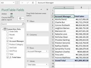


From the above caption, we can see the Total Sales by Account Manager
Create CALCULATE DAX Measure
We wan to create a DAX Measure to return the Total Sales value for Abiola David
- Execute ALT + Tab to return to the Data Model
- In the Measure Grid, execute the DAX Formula: Abiola David Sales:=CALCULATE([Total Sales],Transaction_Data[Account Manager]=”Abiola David”)
- Apply Currency Number Format
- Execute ALT + Tab to return to PivotTable Report in Excel
- Drag and drop Abiola David Sales into the Values area below Total Sales
From the caption below, we can see that the result for Abiola David was returned for other Account Managers which is incorrect. This is what the CALCULATE function does: remove filter from the current context.


Create CALCULATE & KEEPFILTERS DAX Measure
We want other Account Manager to be empty whereas we want to see the Total Sales for Abiola David alone. This is where the KEEPFILTERS comes in which we are going to wrap inside the CALCULATE DAX Function
- Execute ALT + Tab to return to the Data Model
- In the Measure Grid, execute the DAX Formula: Abiola David New Sales:=CALCULATE([Total Sales],KEEPFILTERS(Transaction_Data[Account Manager]=”Abiola David”))
- Apply Currency Number Format
- Execute ALT + Tab to return to PivotTable Report in Excel
- Drag and drop Abiola David New Sales into the Values area below Abiola David Sales
From the caption below, we can see that we have Total Sales for Abiola David alone while other Account Managers are empty. This is exactly want we want to achieve. The KEEPFILTERS wrapped inside the CALCULATE modified the behavior of the CALCULATE. This is a SINGLE COLUMN FILTER


DAX Measure For Multiple Column Filter
Having seen the result for Abiola David alone, we wan to see the results for the following three Account Managers: Natasha Love, Tina John & Nicholas Dean respectively
- Execute ALT + Tab to return to the Data Model
- In the Measure Grid, execute the DAX Formula: Three Account Managers:=CALCULATE([Total Sales],KEEPFILTERS(FILTER(ALL(Transaction_Data),[Account Manager]=”Natasha Love” || [Account Manager]=”Tina John” || [Account Manager]=”Nicholas Dean”)))
- Apply Currency Number Format
- Execute ALT + Tab to return to PivotTable Report in Excel
- Drag and drop Three Account Managers into the Values area below Abiola David New Sales
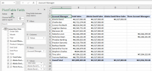
From the caption below, we can see that we have Total Sales for all the three (3) Account Managers alone while the others are empty


See you in the next blog post
